When can a leaf-wax record support a precipitation-isotope claim?

This vignette works through a common problem: a leaf-wax record shows a downcore change, and we want to know whether that change supports a claim about precipitation isotopes. The package reconstructs d2H_precip from measured d2H_wax, then asks whether two time intervals differ by more than the calibration and analytical noise.

The examples use two Iso2k records with different signal sizes and sampling structures. Both use C29 n-alkane d2H_wax, the compound class used by the calibration. The package includes small CSV extracts with finite C29 rows from the source LiPD files. The extraction script is in data-raw/.

Package file	Iso2k record	Source study	Data archive
`LS13WASU_C29_d2H.csv`	LS13WASU, LiPD	Wang et al. (2013), doi:10.1177/0959683613486941	Iso2k LiPD source
`LS14LASO_C29_d2H.csv`	LS14LASO, LiPD	Lauterbach et al. (2014), doi:10.1177/0959683614534741	PANGAEA, doi:10.1594/PANGAEA.834963

The Iso2k compilation is archived at doi:10.25921/57j8-vs18.

detect_change() uses this per-sample detection threshold:

$\mathrm{threshold}_{\mathrm{precip}} = \frac{1.96 \sqrt{2(1 - \rho_t)}\, \sqrt{\sigma_{\mathrm{residual}}^2 + \sigma_{\mathrm{analytical}}^2}}{\beta_{\mathrm{eff}}}$

Here rho_t is the lag-1 temporal autocorrelation, sigma_residual is the calibration residual SD on the wax scale, sigma_analytical is the analytical uncertainty on the wax measurements, and beta_eff is the local effective slope. The threshold is the smallest d2H_precip difference between two independent samples at the site that can be distinguished from within-record noise at 95 percent confidence. The spatial GP intercept is shared by all samples from the same site, so it cancels when the package compares two intervals from one record.

1. Load both records

library(leafwax)

example_record_path <- function(filename) {
  installed_path <- system.file(
    "extdata", "example_records", filename,
    package = "leafwax"
  )
  if (nzchar(installed_path)) {
    return(installed_path)
  }

  source_paths <- file.path(
    c("inst", file.path("..", "inst")),
    "extdata", "example_records", filename
  )
  source_path <- source_paths[file.exists(source_paths)][1]
  if (!is.na(source_path)) {
    return(source_path)
  }

  stop("Could not locate example record: ", filename, call. = FALSE)
}

sugan_path <- example_record_path("LS13WASU_C29_d2H.csv")
sugan <- read.csv(sugan_path)
sugan$d2h_wax <- sugan$d2H_wax
sugan$age     <- sugan$age_yrBP

sonk_path <- example_record_path("LS14LASO_C29_d2H.csv")
sonk <- read.csv(sonk_path)
sonk$d2h_wax <- sonk$d2H_wax
sonk$age     <- sonk$age_yrBP

c(sugan_n        = nrow(sugan),
  sugan_range_pm = round(diff(range(sugan$d2h_wax)), 1),
  sonk_n         = nrow(sonk),
  sonk_range_pm  = round(diff(range(sonk$d2h_wax)), 1))
#>        sugan_n sugan_range_pm         sonk_n  sonk_range_pm 
#>           78.0           31.0           98.0          107.3

Lake Sugan is at 38.8667° N, 93.95° E (2,800 m) in the Qaidam Basin. Sonk11D is at 41.7939° N, 75.1961° E (3,016 m) in the Central Tian Shan. In these extracts, Sugan spans -57 to 1657 yr BP, and Sonk11D spans -45 to 5989 yr BP.

2. Plot the wax records

First inspect the measured d2H_wax values and the interval boundaries used below.

op <- par(mfrow = c(2, 1), mar = c(4.5, 5.4, 2.2, 1), mgp = c(3.4, 0.8, 0))

wax_ylim <- extendrange(c(sugan$d2h_wax, sonk$d2h_wax), f = 0.05)

plot_wax <- function(record, title, boundary, ylim) {
  ord <- order(record$age)
  plot(
    record$age[ord],
    record$d2h_wax[ord],
    type = "o", pch = 16, col = "black",
    xlim = rev(range(record$age)),
    ylim = ylim,
    xlab = "Age (yr BP)",
    ylab = expression(delta^2 * H[wax] ~ "(‰)"),
    main = title
  )
  abline(v = boundary, lty = 2, col = "red")
}

plot_wax(sugan, "Lake Sugan (LS13WASU, C29 n-alkane)",
         boundary = 800, ylim = wax_ylim)
plot_wax(sonk, "Sonk11D (LS14LASO, C29 n-alkane)",
         boundary = 5000, ylim = wax_ylim)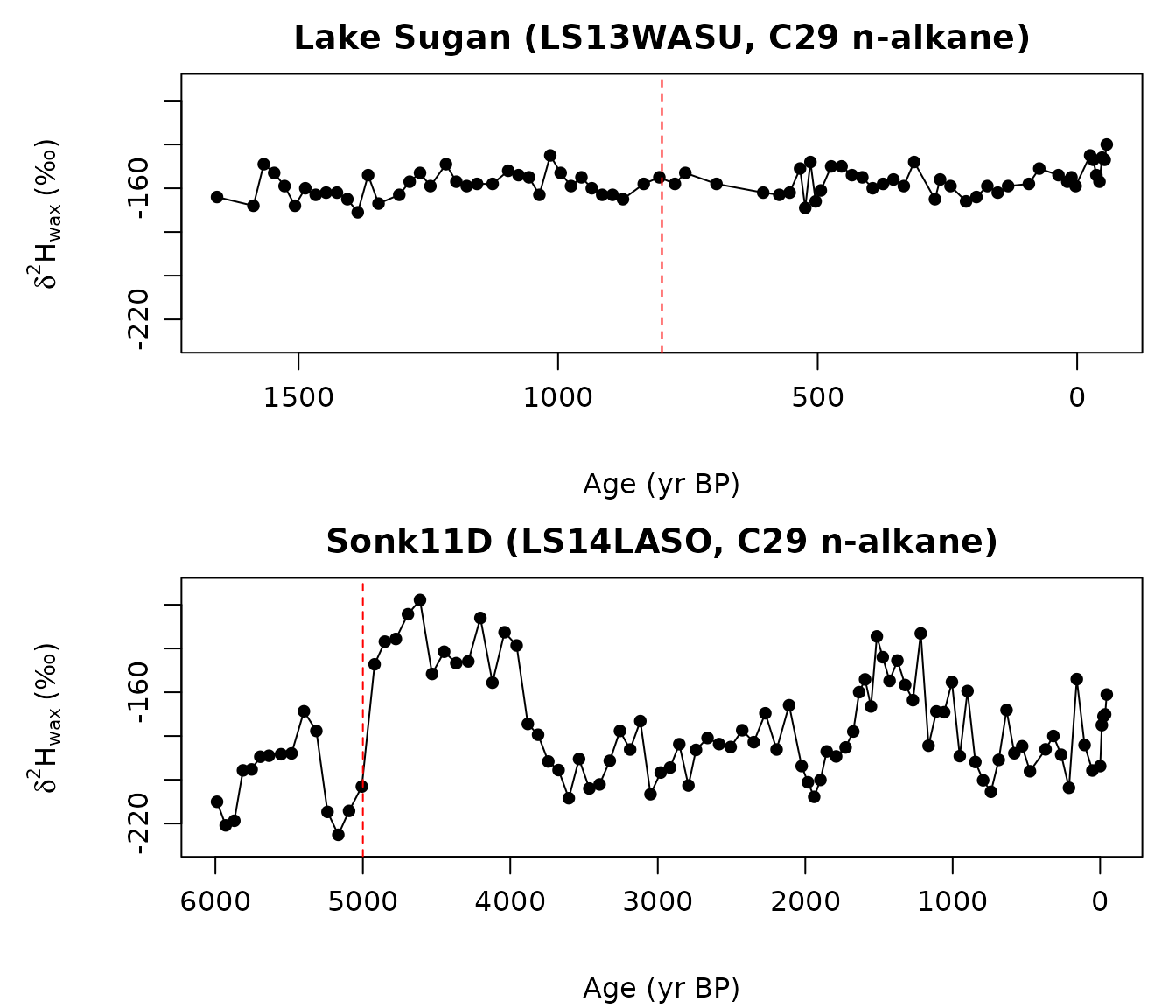


par(op)

The dashed red lines mark the interval boundaries used later for change detection and claim assessment.

3. Claim levels used by `assess_claim()`

assess_claim() reports the highest claim level supported by the record and the evidence supplied by the user. A level can pass only if all lower levels pass.

Level	Claim being made	What must be shown
1	Wax `d2H` changed between two intervals.	The interval-mean wax contrast exceeds analytical uncertainty at the chosen confidence level, after the requested `rho_t` adjustment.
2	The wax change is consistent with directional hydroclimate change.	Level 1 passes and `corroborating_proxies` contains named, non-empty evidence.
3	The record supports a quantitative `d2H_precip` magnitude.	Level 2 passes, a defended `beta_eff` is supplied, the full inversion posterior is available, and the posterior probability of exceeding `magnitude_precip` meets the requested confidence level.
4	The quantitative magnitude can be attributed to precipitation isotopes.	Level 3 passes and independent evidence supports stationary vegetation, source-water seasonality, and evapotranspirative enrichment over the interval.

The function checks that the required evidence fields are present. It does not decide whether the proxy interpretation or stationarity argument is scientifically adequate. That still requires record-specific evidence and citations.

4. Local effective slope

local_effective_slope() returns one slope value for each posterior draw at the site. Each value combines the global beta_oipc draw with the spatial slope GP. The function returns the model draws directly; it does not cap or filter them. Passing the full vector to invert_d2H() carries slope uncertainty into the reconstruction. Passing one number, such as the posterior median, gives a point-slope sensitivity run.

The examples below use baseline_sp (spatial intercepts + slope GP, no environmental predictors) for simplicity. baseline_env_sp is the companion variant whose detection thresholds appear in Figure 5 of the accompanying manuscript (Bradley 2026); switching model_name is the only change needed to use it.

sugan_lon <- 93.95;   sugan_lat <- 38.8667
sonk_lon  <- 75.1961; sonk_lat  <- 41.7939

slope_sugan <- suppressWarnings(local_effective_slope(
  longitude = sugan_lon, latitude = sugan_lat,
  model_name = "baseline_sp", n_draws = 100,
  verbose = FALSE
))

slope_sonk <- suppressWarnings(local_effective_slope(
  longitude = sonk_lon, latitude = sonk_lat,
  model_name = "baseline_sp", n_draws = 100,
  verbose = FALSE
))

rbind(
  sugan = quantile(slope_sugan, c(0.025, 0.5, 0.975)),
  sonk  = quantile(slope_sonk,  c(0.025, 0.5, 0.975))
)
#>            2.5%       50%     97.5%
#> sugan 0.2453382 0.3878862 0.5338104
#> sonk  0.3050322 0.4423601 0.5633999

5. Invert wax values to precipitation values

invert_d2H() uses the slope vector from the previous section. The record_id argument tells the function that all rows belong to one downcore record. return_full = TRUE keeps the posterior draws needed by detect_change().

The inversion samples analytical uncertainty and the model residual SD. For contrasts within one record, the spatial GP intercept cancels because each sample uses the same site-level intercept draw.

recon_sugan <- suppressWarnings(invert_d2H(
  d2H_wax    = sugan$d2h_wax,
  d2H_wax_sd = rep(3, nrow(sugan)),
  longitude  = rep(sugan_lon, nrow(sugan)),
  latitude   = rep(sugan_lat, nrow(sugan)),
  model_name = "baseline_sp",
  n_posterior_draws = 100,
  slope        = slope_sugan,
  record_id    = "LS13WASU",
  return_full  = TRUE,
  verbose      = FALSE
))

recon_sonk <- suppressWarnings(invert_d2H(
  d2H_wax    = sonk$d2h_wax,
  d2H_wax_sd = rep(3, nrow(sonk)),
  longitude  = rep(sonk_lon, nrow(sonk)),
  latitude   = rep(sonk_lat, nrow(sonk)),
  model_name = "baseline_sp",
  n_posterior_draws = 100,
  slope        = slope_sonk,
  record_id    = "LS14LASO",
  return_full  = TRUE,
  verbose      = FALSE
))

6. Detection threshold and posterior probability of change

detect_change() compares the interval-mean d2H_precip draws between two time intervals. For each posterior draw, it subtracts the baseline interval mean from the test interval mean. It returns a detection threshold and the posterior probability that the interval difference exceeds target magnitudes. The example uses sigma_residual = 16, the residual scale used in the package’s spatial-model examples. For an analysis, use the residual SD from the calibration being propagated.

estimate_temporal_autocorrelation() estimates lag-1 autocorrelation after ordering the record by age and subtracting a flat mean. This AR(1) estimate is simple and transparent for nearly regular records. Irregular paleo records need sensitivity tests or a method for uneven sampling. Change-point tools such as bcp and Rbeast answer a different question: they can test whether a boundary or trend is supported, but they do not estimate the rho_t term in the detection-threshold formula. A Lomb-Scargle option is planned for v0.3 (method = "lomb_scargle").

The Sugan example compares the last eight centuries with the older part of the record; its wax contrast is small. The Sonk11D example compares 4-5 ka with 5-6 ka, where the extracted C29 n-alkane series has a much larger contrast.

rho_sugan <- estimate_temporal_autocorrelation(
  sugan$d2h_wax, sugan$age, method = "ar1"
)

dc_sugan <- detect_change(
  reconstruction    = recon_sugan,
  age               = sugan$age,
  baseline_interval = c(-100, 800),
  test_intervals    = list(older = c(800, 1700)),
  sigma_residual    = 16,
  sigma_analytical  = 3,
  rho_t             = rho_sugan,
  beta_eff          = stats::median(slope_sugan),
  confidence        = 0.95,
  magnitudes        = c(10, 30, 50)
)
#> Warning: leafwax preview posteriors in use (detect_change): 100 draws of
#> 'baseline_sp'. Tail probabilities and 95% credible intervals are unstable at
#> this sample size; not suitable for inference. Run
#> download_model_data("baseline_sp") for the full posterior.

rho_sonk <- estimate_temporal_autocorrelation(
  sonk$d2h_wax, sonk$age, method = "ar1"
)

dc_sonk <- detect_change(
  reconstruction    = recon_sonk,
  age               = sonk$age,
  baseline_interval = c(4000, 5000),
  test_intervals    = list(early_holocene = c(5000, 6000)),
  sigma_residual    = 16,
  sigma_analytical  = 3,
  rho_t             = rho_sonk,
  beta_eff          = stats::median(slope_sonk),
  confidence        = 0.95,
  magnitudes        = c(10, 30, 50)
)
#> Warning: leafwax preview posteriors in use (detect_change): 100 draws of
#> 'baseline_sp'. Tail probabilities and 95% credible intervals are unstable at
#> this sample size; not suitable for inference. Run
#> download_model_data("baseline_sp") for the full posterior.

list(
  sugan = list(rho_t = round(rho_sugan, 3),
               threshold_permil = round(dc_sugan$threshold, 1),
               intervals        = dc_sugan$intervals),
  sonk = list(rho_t = round(rho_sonk, 3),
              threshold_permil = round(dc_sonk$threshold, 1),
              intervals        = dc_sonk$intervals)
)
#> $sugan
#> $sugan$rho_t
#> [1] 0.203
#> 
#> $sugan$threshold_permil
#> [1] 103.8
#> 
#> $sugan$intervals
#>   interval n_baseline n_test delta_mean delta_median delta_lower delta_upper
#> 1    older         41     37  -9.301603    -7.864667   -31.47903    8.930941
#>   p_abs_delta_gt_10 p_abs_delta_gt_30 p_abs_delta_gt_50
#> 1              0.48              0.04              0.01
#> 
#> 
#> $sonk
#> $sonk$rho_t
#> [1] 0.716
#> 
#> $sonk$threshold_permil
#> [1] 54.4
#> 
#> $sonk$intervals
#>         interval n_baseline n_test delta_mean delta_median delta_lower
#> 1 early_holocene         12     15  -137.2436    -137.8394   -200.0781
#>   delta_upper p_abs_delta_gt_10 p_abs_delta_gt_30 p_abs_delta_gt_50
#> 1    -94.7102                 1                 1                 1

The two records differ. Sugan has lag-1 autocorrelation 0.2, a 95 percent detection threshold of about 104 per mil, and posterior probability 0.04 for a 30 per mil shift. Sonk11D has lag-1 autocorrelation 0.72, a threshold of about 54 per mil, and posterior probability 1.00 for a 30 per mil shift.

In this example, the Sugan contrast is too small relative to calibration noise. The Sonk11D contrast is large enough for the 30 per mil quantitative claim to pass the posterior-probability test.

7. Assess a claim

The next chunk asks whether each record supports a Level 4 claim of a 30 per mil d2H_precip change. The evidence strings are placeholders that show the required API structure. They do not replace a record-specific literature review.

build_claim <- function(beta_eff, rho_t, baseline, test, magnitude_precip) {
  list(
    level             = 4,
    interval_baseline = baseline,
    interval_test     = test,
    sigma_analytical  = 3,
    rho_t             = rho_t,
    confidence        = 0.95,
    beta_eff          = beta_eff,
    magnitude_precip  = magnitude_precip,
    corroborating_proxies = list(
      regional_proxy = "regional records show coeval shift"
    ),
    vegetation_stationary = list(
      value    = TRUE,
      evidence = "n-alkane chain length distributions stable across the boundary"
    ),
    seasonal_source_stationary = list(
      value    = TRUE,
      evidence = "regional d18O record shows no seasonality shift"
    ),
    evapotranspirative_stationary = list(
      value    = TRUE,
      evidence = "leaf-water proxy stable; no aridity transition"
    )
  )
}

sugan_record <- data.frame(
  d2h_wax     = sugan$d2h_wax,
  age         = sugan$age,
  d2h_wax_err = rep(3, nrow(sugan))
)
sonk_record <- data.frame(
  d2h_wax     = sonk$d2h_wax,
  age         = sonk$age,
  d2h_wax_err = rep(3, nrow(sonk))
)

verdict_sugan <- suppressWarnings(assess_claim(
  record         = sugan_record,
  claim          = build_claim(stats::median(slope_sugan),
                                rho_sugan,
                                c(-100, 800), c(800, 1700),
                                magnitude_precip = 30),
  reconstruction = recon_sugan
))

verdict_sonk <- suppressWarnings(assess_claim(
  record         = sonk_record,
  claim          = build_claim(stats::median(slope_sonk),
                                rho_sonk,
                                c(4000, 5000), c(5000, 6000),
                                magnitude_precip = 30),
  reconstruction = recon_sonk
))

c(sugan_highest_level  = verdict_sugan$highest_level,
  sugan_supported_at_4 = verdict_sugan$asserted_supported,
  sonk_highest_level   = verdict_sonk$highest_level,
  sonk_supported_at_4  = verdict_sonk$asserted_supported)
#>  sugan_highest_level sugan_supported_at_4   sonk_highest_level 
#>                    0                    0                    4 
#>  sonk_supported_at_4 
#>                    1

Read verdict$levels from top to bottom. Each row reports whether a level passed and, if it failed, why. In this run, Sugan fails at the wax-change step. Sonk11D clears Level 4 because the interval contrast is large and the example supplies stationarity evidence. The stationarity strings are placeholders; a real Level 4 claim needs record-specific evidence and citations.

8. Plot the reconstructions

op <- par(mfrow = c(2, 1), mar = c(4.5, 5.4, 2.2, 1), mgp = c(3.4, 0.8, 0))

precip_ylim <- extendrange(
  c(recon_sugan$summary$d2h_precip_lower,
    recon_sugan$summary$d2h_precip_upper,
    recon_sonk$summary$d2h_precip_lower,
    recon_sonk$summary$d2h_precip_upper),
  f = 0.05
)

plot_recon <- function(rec, ages, title, boundary, ylim) {
  ord <- order(ages)
  plot(
    ages[ord],
    rec$summary$d2h_precip_median[ord],
    type = "n",
    xlim = rev(range(ages)),
    ylim = ylim,
    xlab = "Age (yr BP)",
    ylab = expression(delta^2 * H[precipitation] ~ "(‰)"),
    main = title
  )
  polygon(
    c(ages[ord], rev(ages[ord])),
    c(rec$summary$d2h_precip_lower[ord],
      rev(rec$summary$d2h_precip_upper[ord])),
    border = NA, col = adjustcolor("steelblue", alpha.f = 0.3)
  )
  lines(ages[ord], rec$summary$d2h_precip_median[ord],
        type = "o", pch = 16, col = "black")
  abline(v = boundary, lty = 2, col = "red")
}

plot_recon(recon_sugan, sugan$age,
           "Lake Sugan (LS13WASU): small interval contrast",
           boundary = 800, ylim = precip_ylim)
plot_recon(recon_sonk, sonk$age,
           "Sonk11D (LS14LASO): large 4-6 ka contrast",
           boundary = 5000, ylim = precip_ylim)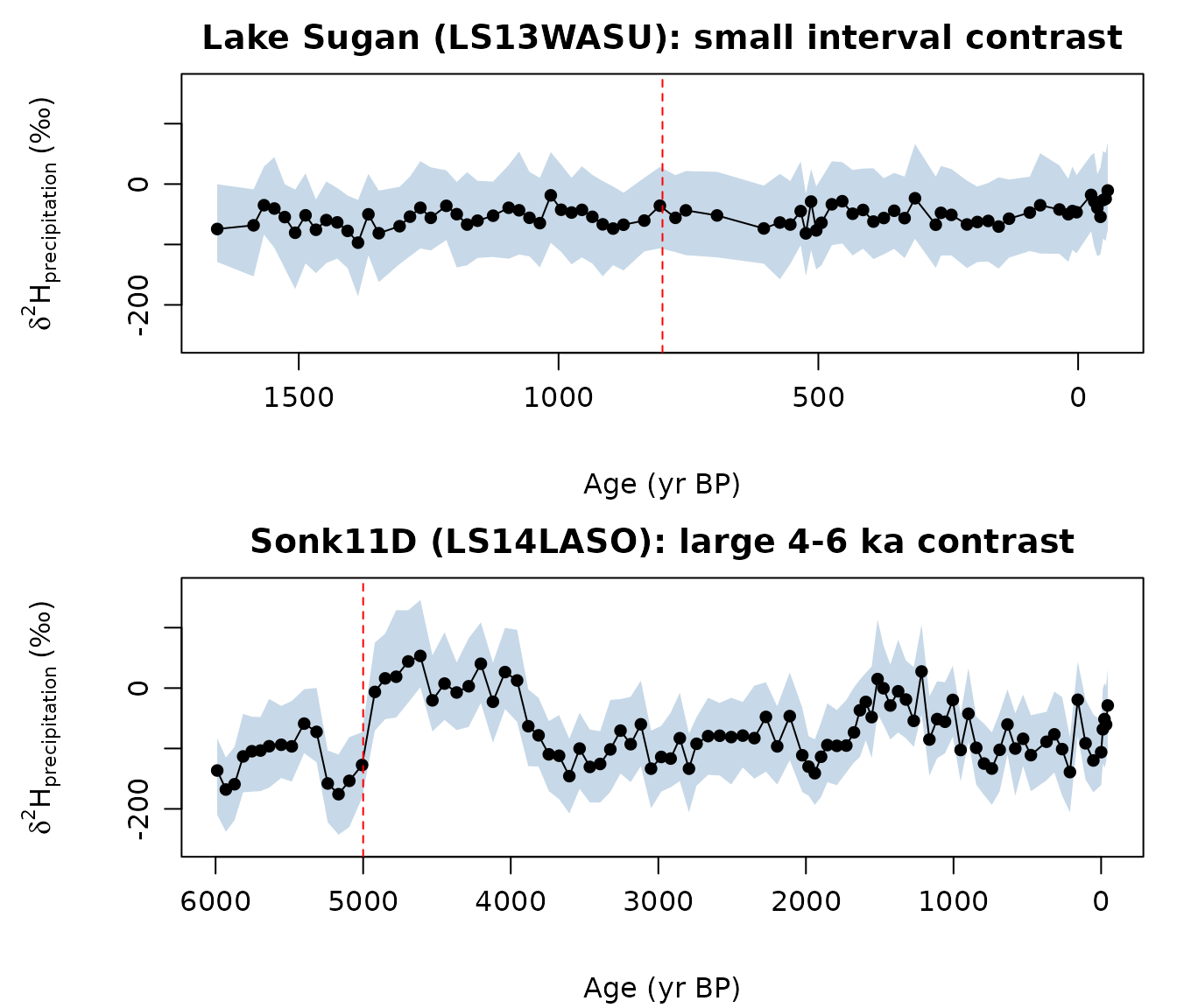


par(op)

The shaded band is the 90 percent credible interval for each sample. It includes analytical uncertainty, regression-parameter uncertainty, the local slope posterior, and the calibration residual SD. The dashed red line marks the interval boundary used above.

Takeaway

A record’s ability to support a d2H_precip claim depends on three quantities: the interval-mean d2H_wax contrast relative to sigma_residual, the local effective slope, and lag-1 temporal autocorrelation. detect_change() combines these into a threshold and a posterior probability. assess_claim() then checks the result against the four claim levels. Small contrasts can fail at the first step. Large contrasts can support directional and quantitative claims, but a Level 4 claim still requires independent evidence for stationarity.

Notes

The vignette uses 100 posterior draws so it runs quickly. For final reconstructions, use the full posterior by omitting n_draws and n_posterior_draws.
estimate_temporal_autocorrelation() uses a flat-mean lag-1 estimator and works best for nearly regular spacing. For irregular paleo records, use sensitivity analyses or an uneven-sampling autocorrelation method for rho_t. Use bcp or Rbeast for complementary change-point or trend checks, not as direct rho_t estimators.